My UCAS coursework may not be reproduced without permission! My UCAS coursework may not be reproduced without permission! My UCAS coursework may not be reproduced without permission!
# Introduction
Graphs are commonly used information carriers in complex systems and can represent many complex relationships in reality, such as social networks, criminal networks, transportation networks, etc. As a kind of non-Euclidean data, graph structure is difficult to directly apply deep learning methods such as convolutional neural network (CNN) and recurrent neural network (RNN).
To construct feature representations for graph data mining, graph embedding maps nodes into a low-dimensional space, generating low-dimensional vectors that preserve some important information in the original graph. Currently, graph embeddings are not only successful in machine learning tasks on complex networks such as node classification, link prediction, node clustering, and visualization, but are also widely used in real-world tasks such as social influence modeling and content recommendation. Early graph embedding algorithms were mainly used for data dimensionality reduction, building similarity graphs through neighborhood relationships, embedding nodes in low-dimensional vector space, and maintaining the similarity of connected node vectors. Such methods usually have high time complexity and are difficult to scale to large graphs. In recent years, graph embedding algorithms have turned to scalable methods. For example, the matrix factorization method uses an approximate decomposition of the adjacency matrix as the embedding; the random walk method inputs the walk sequence into Skip-Gram to generate the embedding. These methods exploit the sparsity of the graph to reduce time complexity.
In order to adapt to better downstream tasks, good embedding methods need to meet more requirements. The main challenges at present are:
(1) Need to ensure that the embedding describes the properties of the graph well. They need to represent graph topology, node connections, and node neighborhoods. The performance of a prediction or visualization depends on the quality of the embedding.
(2) The size of the network should not slow down the embedding process. Graphs are often very large, for example a common social network may have millions of interactions, so good embedding methods need to be efficient on large graphs.
(3) Longer embedding dimensions can retain more information, but at the same time it will bring higher time and space complexity, and users need to make trade-offs according to their needs.
# Image embedding
In order to transform the graph from the original graph space to the embedding space, different models can be used to merge different types of information. Commonly used models mainly include matrix decomposition, random walk, and deep neural network.
# Graph embedding based on matrix factorization
Adjacency matrices are often used to represent the structure of graphs, where each column and row represents a node, and the matrix entries represent the relationships between nodes. You can simply use row vectors or column vectors as vector representations of nodes, but the resulting representation space is N-dimensional, where N is the total number of nodes. Graph embedding aims to learn the low-dimensional vector space of the network, ultimately finding a low-rank space to represent the network. While matrix factorization methods have the same goal of learning the low-rank space of the original matrix, among a series of matrix factorization models, singular value decomposition (SVD) is often used for graph embedding due to its optimality for low-rank approximation, and non-negative matrix factorization is often used for its advantages as an additive model.
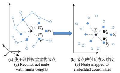
Locally linear embedding (LLE) represents each node as a linear combination of adjacent nodes and constructs a neighborhood-preserving mapping. The specific implementation is divided into three steps: (1) Select k neighboring nodes using a certain metric (such as Euclidean distance); (2) Reconstruct the nodes linearly weighted by k neighbors and minimize the node reconstruction error to obtain the optimal weight; (3) Minimize the objective function constructed by the optimal weight to generate Y. However, this model is very sensitive to the choice of k value, which has a great impact on the final dimensionality reduction result.

Laplacian eigenmaps (LE) are similar to LLE in that they also construct relationships between data from the perspective of local approximation. LE uses an adjacency matrix to build an embedding representation that contains local structural information and requires connected nodes to be as close as possible in the embedding space.
The objective function of LE emphasizes node pairs with large weights and weakens node pairs with small weights, causing the local topology in the original graph to be destroyed. In order to enhance the local topology preservation of graph embedding, Cauchy graph embedding (CGE) introduces the inverse function of distance to maintain the similarity relationship of nodes in the embedding space. Compared with LE, the objective function of CGE emphasizes short distances, that is, ensuring that the closer the locally adjacent nodes are, the closer the distance in the embedding space is.
In response to the current demand for dynamic graph analysis, a more general dynamic graph embedding method based on matrix decomposition has emerged. DANE adopts a distributed framework: in the offline part, using the method of maximizing correlation, introducing and to maximize the correlation after projection of topological embedding and feature embedding, capturing the dependence of the graph structure and node attributes, and then splicing the first d eigenvectors to keep and consistent in representation; in the online part, matrix perturbation theory is used to update the embedded eigenvalues and eigenvectors. At time t, DANE performs spectral graph embedding on the topology structure and node attributes; at time t+1, DANE uses matrix perturbation theory to update and to generate new embeddings.
# Graph embedding based on random walk
Inspired by word2vec, the random walk-based graph embedding method converts nodes into words, uses random walk sequences as sentences, and uses graph Skip-Gram to generate embedding vectors of nodes. The random walk method can preserve the structural characteristics of the graph and still perform well on large graphs that cannot be completely observed.
DeepWalk generates embeddings using a random walk that starts at a selected node and moves from the current node to random neighbors and continues for a specified number of steps. The process consists of three steps as shown in Figure 2.

(1) Sampling: Sampling the graph through random walks. Perform few random walks from each node. The authors show that it is sufficient to perform 32 to 64 random walks from each node, and the authors show that the length of a good random walk is about 40 steps.
(2) Training skip-gram: Random walk is equivalent to sentences in word2vec method. The Skip-gram network accepts a node in a random walk as a one-hot vector as input and maximizes the probability of predicting neighbor nodes. It is usually trained to predict about 20 neighbor nodes (10 nodes to the left, 10 nodes to the right).
(3) Calculate embedding: Embedding is the output of the hidden layer of the network. DeepWalk computes the embedding of each node in the graph.
The DeepWalk method randomly performs a random walk, which means that the embedding does not preserve the local neighborhood of nodes well. The Node2vec approach solves this problem. Node2vec is an improved version of DeepWalk with very small differences in random walks. It has parameters P and Q. The parameter Q defines how likely the random walk is to discover undiscovered parts of the graph, while the parameter P defines how likely the random walk is to return to the previous node. The parameter P controls the discovery of microscopic views around the node. The parameter Q controls the discovery of larger neighborhoods. It infers communities and complex dependencies.

Figure 3 shows the probability of a random walk step in Node2vec. Taking a step from a red node to a green node, the probability of returning to a red node is 1/P, while the probability of going to a node not connected to the previous (red) node is 1/Q, and the probability of going to a neighbor of a red node is 1.
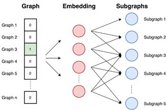
Graph2vec is based on the idea of the doc2vec method using skip-gram network, which takes the ID of the document on the input and is trained to maximize the probability of predicting random words from the document. Since the task is to predict subgraphs, graphs with similar subgraphs and similar structures have similar embeddings. As shown in Figure 4, the Graph2vec method consists of three steps.

(1) Sample and relabel all subgraphs in the graph. A subgraph is a set of nodes that appear around a selected node, and the nodes in the subgraph are no further apart than the selected number of edges.
(2) Train the skip-gram model. Diagrams are similar to documents. Since a document is a collection of words, a graph is a collection of subgraphs. At this stage, the skip-gram model is trained. It is trained to maximize the probability of predicting subgraphs present in the input graph. The input graph is provided as one-hot vectors.
(3) Compute the embedding by providing the graph ID as a one-hot vector at the input, the embedding is the result of the hidden layer.
# Graph embedding based on graph neural network
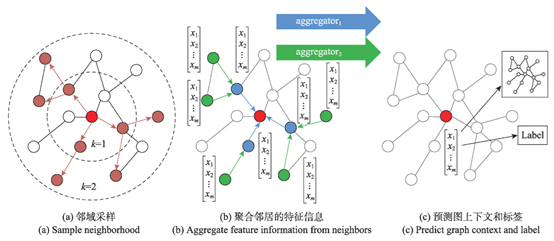
GCN is usually applied to direct push representation learning of fixed graphs. GraphSAGE extends it to the task of inductive unsupervised learning, using node features (such as text attributes, node degrees) to learn embedded representations of invisible nodes. As shown in Figure 5, GraphSAGE does not train a separate embedding for each node, but trains an aggregator function by sampling and aggregating the local neighborhood features of the node, while learning the topology and feature distribution of each node’s neighborhood to generate an embedding representation. Compared with GCN, GraphSAGE uses an unsupervised loss function to force nearby nodes to have similar representations and distant nodes to have different representations. Given downstream tasks, GraphSAGE can replace or add the corresponding objective function to perform supervised or semi-supervised learning to improve the flexibility of the model; the training process performs batch training to improve the convergence speed of the model.

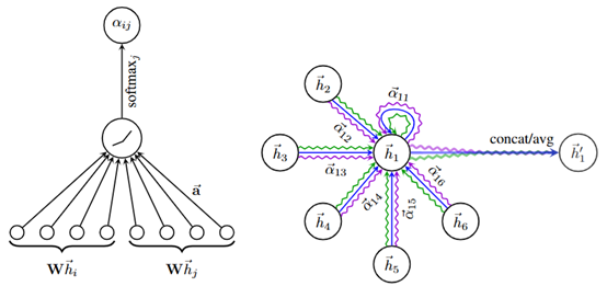
As shown in Figure 6, graph attention network (GAT) introduces an attention mechanism based on GCN, weights and sums the features of neighboring nodes, and assigns different weights. For a single node, GAT uses self-attention to obtain the attention coefficient, uses masked-attention to allocate attention to the neighborhood of node i, and uses multi-head attention to generate node embeddings.
The attention parameters are shared throughout the graph, which greatly reduces the storage space occupied by the parameters. At the same time, GAT samples all neighbor nodes, which is more representative than the embedding obtained by GraphSAGE. The disadvantage of GAT is that when using second-order or higher neighbors, it can easily lead to over-smoothing.

# Summary and discussion
Graph embedding can be interpreted as generating vector representations of graph data that are used to gain insight into certain properties of the graph. Table 1 summarizes the main graph embedding model strategies and summarizes the shortcomings of each model.
Table 1 Summary of model strategies
| Categories | Models | Strategies | Disadvantages |
|---|---|---|---|
| Matrix decomposition | LLE | Construct neighborhood-preserving mapping and minimize the reconstruction loss function | Very sensitive to the choice of k value, affecting the dimensionality reduction results |
| LE | Keep connected nodes as close as possible in the embedding space | It is difficult to learn the local topology in the original graph | |
| DANE | Laplacian eigenmap captures the structure and attribute information at time t, and matrix perturbation theory updates dynamic information | The online part does not consider the high-order similarity of the graph | |
| Random walk | Deepwalk | Using random walk to sample nodes, Skip-Gram maximizes node co-occurrence probability | Embedding does not preserve the local neighborhood of nodes well. |
| node2vec | Introducing a biased random walk based on Deepwalk | Does not distinguish between node or relationship types | |
| Graph2vec | Use skip-gram network to maximize the probability of predicting random words from documents | Use adjacent nodes and do not consider high-order similarity information of the graph. | |
| Graph Neural Network | GraphSAGE | Sampling and aggregating local neighborhood features of nodes to train aggregator functions | Only aggregating neighbor information makes it difficult to capture complex neighbor relationships and graph structures |
| GAT | Introduce self-attentio and multi-head attention based on GCN | When using second-order or above neighbors, it is easy to cause over-smoothing |
The main task at this stage is still to improve the scalability of the model to large-scale and complex graph data, innovate model methods and improve the performance of downstream tasks.
Personally, I believe that task-specific embeddings still have strong research significance. The results generated by most graph embedding models will be used for multiple tasks such as node classification, link prediction, and visualization. But for specific downstream tasks, different graph embedding models have different effects on downstream tasks. Task-oriented embedding models can only focus on one task and make full use of information related to the task to train the model.
My UCAS coursework may not be reproduced without permission! My UCAS coursework may not be reproduced without permission! My UCAS coursework may not be reproduced without permission!
References:
[1] Yuan Lining, Li Xin, Wang Xiaodong, & Liu Zhao. (2022). Review of graph embedding models. Journal of Frontiers of Computer Science & Technology, 16(1).
[2] Roweis, S. T., & Saul, L. K. (2000). Nonlinear dimensionality reduction by locally linear embedding. science, 290(5500), 2323-2326.
[3] Belkin, M., & Niyogi, P. (2001). Laplacian eigenmaps and spectral techniques for embedding and clustering. Advances in neural information processing systems, 14.
[4] Perozzi, B., Al-Rfou, R., & Skiena, S. (2014, August). Deepwalk: Online learning of social representations. In Proceedings of the 20th ACM SIGKDD international conference on Knowledge discovery and data mining (pp. 701-710).
[5] Grover, A., & Leskovec, J. (2016, August). node2vec: Scalable feature learning for networks. In Proceedings of the 22nd ACM SIGKDD international conference on Knowledge discovery and data mining (pp. 855-864).
[6] Narayanan, A., Chandramohan, M., Venkatesan, R., Chen, L., Liu, Y., & Jaiswal, S. (2017). graph2vec: Learning distributed representations of graphs. arXiv preprint arXiv:1707.05005.
[7] Hamilton, W., Ying, Z., & Leskovec, J. (2017). Inductive representation learning on large graphs. Advances in neural information processing systems, 30.
[8] Veličković, P., Cucurull, G., Casanova, A., Romero, A., Lio, P., & Bengio, Y. (2017). Graph attention networks. arXiv preprint arXiv:1710.10903.
[9] Cai, H., Zheng, V. W., & Chang, K. C. C. (2018). A comprehensive survey of graph embedding: Problems, techniques, and applications. IEEE transactions on knowledge and data engineering, 30(9), 1616-1637.
[10] Cui, P., Wang, X., Pei, J., & Zhu, W. (2018). A survey on network embedding. IEEE transactions on knowledge and data engineering, 31(5), 833-852.
