This article is my UCAS course paper reading report and is not allowed to be reproduced! ! !

This article is my UCAS course paper reading report and is not allowed to be reproduced! ! !

This article is my UCAS course paper reading report and is not allowed to be reproduced! ! !

# Team introduction

# Author of this article

Chunlin Xiong: Postdoctoral fellow at the Shenzhen Institute of Advanced Technology, Chinese Academy of Sciences and Sangfor, mainly researching APT detection and forensic analysis. As the first author, he published a paper Conan: A Practical Real-Time APT Detection System With High Accuracy and Efficiency in the TDSC journal in 2022

Jiacen Xu and Zhou Li: University of California, focusing on domain name system security, log-based anomaly detection, privacy protection, machine learning security and privacy

Fan Yang and Kehuan Zhang: Chinese University of Hong Kong, focusing on binary code security analysis

# Main research teams in the field

In the field of Provenance graph-based detectors for APTs (APT threat detection based on traceability graphs), there are mainly three teams:

• University of Illinois at Chicago team: This team proposed SLEUTH in USENIX’17, which applies traceability graphs to the field of APT attack detection. Poirot was proposed at the 2019 CCS conference and Holmes was proposed at S&P'19. This method combines the Kill Chain and ATT&CK frameworks. In addition, in 2021 EurS&P proposes Extrator and introduces external knowledge.

• University of Illinois at Urbana-Champaign team: This team proposed UNICORN and ProvDetector respectively at NDSS’20, and also proposed RapSheet at S&P in 2020, which integrates the ATT&CK framework.

*Purdue University team: The core results of this team include BEEP proposed by NDSS'13, ProTracer proposed by NDSS'16 and ATLAS proposed by USENIX'21.

# Topic selection background

The long-standing war between computing system defenses and attacks continues to evolve, and despite the widespread deployment of defenses such as intrusion detection systems (IDS) and anti-malware, sophisticated attacks themed around advanced persistent threats (APTs) are still able to penetrate organizational networks and cause serious damage. The main reasons for failure to defend against APT attacks are:

1. Traditional defense systems rely on attack signatures that attackers can easily change
2. Traditional defense systems do not fully exploit the causal relationships between different entities in a computing system or network to perform detection (e.g., on system logs).

In order to solve these two basic problems, defense systems based on data traceability have recently been developed. Data provenance transforms system logs into graphical representations that capture temporal and causal relationships between different types of entities (e.g., processes and files). On this representation, graph operations such as graph traversal can be performed to detect ongoing attacks or reason about the root cause of an intrusion. With data provenance, it becomes possible to detect APT attacks as the rich contextual information embedded in logs is well utilized.

But all existing traceability-based systems fail to meet all basic deployment requirements in complex production environments, including detection accuracy, runtime efficiency, “signaturelessness” and fine-grainedness.

1. Attribution systems (Atlas, RapSheet, Homles) that rely on signatures, heuristics or known attack traces can be circumvented after attackers adapt their patterns.
2. Some systems choose to build a single traceability graph from the logs and detect malicious entities and events (Shadewatcher), but when a large number of logs need to be analyzed, this overhead becomes too expensive, and a large number of false positives are also generated in such a setting.
3. A few systems build time-ordered snapshots from logs in a streaming manner and try to detect abnormal snapshots (Unicorn), but since analysts must analyze all entities/interactions within the abnormal snapshot, the detection granularity is too rough.

# Data tracing for attack investigation

To enable attack detection and forensics, system logs are typically collected by system-level auditing tools such as Windows ETW, Linux Audit, and FreeBSD Dtrace, which describe interactions between system entities such as processes and processes. document. Logs collected on end hosts within an organization are often analyzed by central services such as Security Information and Event Management (SIEM) to detect sophisticated cross-machine attacks.

In addition to system logs, data sources have been proposed to detect and reason about intrusions, and even long-term Advanced Persistent Threat (APT) attacks involving multiple stages such as reconnaissance, installation, command and control, and lateral movement can be detected. Essentially, data provenance builds a dependency graph from system logs to describe the relationships between events, so detection and investigation can be transformed into graph-related operations.

Of all graph-related operations, graph traversal is probably the most popular choice. A prominent example is backtracking, through which security analysts query a provenance graph with point-of-interest (POI) entities and time windows, and return events with time dependencies. However, this simple approach suffers from “dependency explosion”, which can be caused by long-running processes that interact with many principals/objects during their lifetime.

# Learning-based traceability graph attack detection

In order to accurately locate attack events, a large number of rule-based methods have been proposed, which use the knowledge of known attack behaviors to search the traceability graph. However, writing rules requires considerable effort on the part of the analyst, and attacks in invisible modes may be missed. Therefore, learning-based approaches, which train models with normal system behavior (as well as malicious behavior with supervised learning) to detect anomalous system execution, have recently started to gain more attention. Although applying learning-based methods to capture cyber attacks is not new, provenance graphs introduce new opportunities to exploit graph structures and apply new graph learning methods. Existing work can be classified according to the granularity of the goals: edges/nodes, paths, and graphs.

# Image embedding

To capture key properties of provenance graphs, provenance systems often use graph embeddings. In other fields such as social networks, recommender systems, and life sciences, graph embeddings have achieved significant success in improving the performance of downstream tasks such as graph classification, clustering, and regression. Essentially, graph embeddings learn to represent nodes, edges, subgraphs, or entire graphs with low-dimensional vectors that capture the graph structure, point-to-point relationships, and other relevant information about the graph. The provenance system utilizes two types of graph embedding techniques:

Node embedding maps each node of the graph to a low-dimensional vector that preserves its key information, such as the node’s neighborhood information, the node’s structural role, and the node’s state. Popular node embedding models include DeepWalk, GCN, GraphSage, etc. Downstream tasks such as node classification and edge classification related to node, edge and path based detection can be performed by calculating the node/edge score of the node embedding and comparing it to a threshold.

Full Graph Embedding represents the entire graph with a single vector that aggregates information from node representations. Popular full-graph embedding models include DiffPool, graph2vec, graph sketching, etc. Downstream tasks such as graph classification and clustering related to graph-based detection can be performed through the computation of graph vectors.

Edge embedding has also been proposed for applications such as recommendation in social networks, but it has not been found to be used by any traceability system.

# Method statement

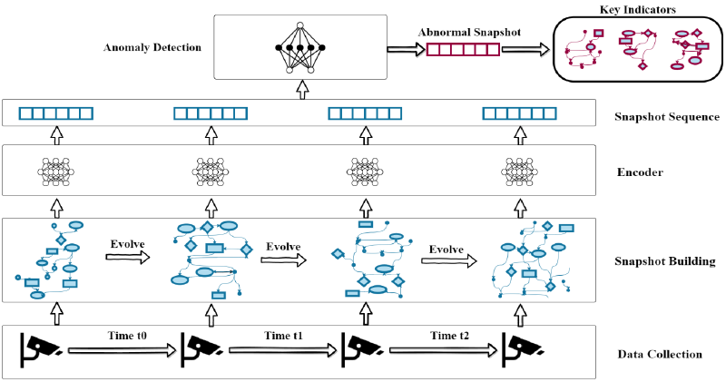
In this paper, the authors propose PROGRAPHER, a new source-based anomaly detection system that simultaneously meets the requirements of detection accuracy, runtime efficiency, “signature-free”, and fine-grainedness. PROGRAPHER performs detection at graph granularity, and when logs are ingested, PROGRAPHER extracts snapshots to reduce the computational and memory costs of the entire source graph. On each snapshot, PROGRAPHER applies a full-graph embedding technique called graph2vec to generate rooted subgraphs (RSGs) as low-dimensional representations of each node, and learns the graph representation by maximizing the co-occurrence likelihood of normal snapshots and normal RSGs. To capture the temporal dynamics between snapshots, a sequence learning model called TextRCNN is employed, thus predicting the representation of future snapshots and detecting anomalous snapshots when they deviate from the prediction. Previous systems like Unicorn were stuck at reporting anomalous snapshots, but PROGRAPHER continues to pinpoint anomalous entities by ranking RSGs and reporting the most suspicious entities as attack indicators.

# Overview

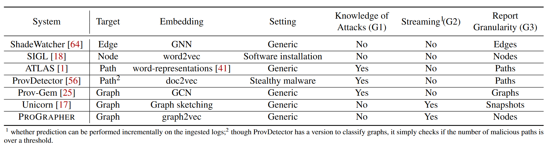
This article envisions PROGRAPHER to achieve three design goals (G1 - G3). It is worth noting that none of the previous methods can meet all these requirements, and we compare PROGRAPHER with other representative methods in Table 1.

G1: PROGRAPHER should learn normal behavior patterns from benign logs, so it increases the chance of detecting attacks that exploit zero-day vulnerabilities. In other words, PROGRAPHER should be built through unsupervised learning without any knowledge of attack or event labels.

G2: Since processing the provenance graph for a long time is very resource-consuming, PROGRAPHER should be able to process subgraphs of the entire provenance graph separated by cycles and exploit the temporal dynamics between cycles for detection.

G3: PROGRAPHER should be able to accurately identify subgraphs with abnormal activity. Additionally, PROGRAPHER should narrow the scope of the investigation by pointing out entities directly related to the attack.

PROGRAPHER consists of four components to satisfy G1-G3:

1. Snapshot Builder

2. Encoder

3. Anomaly detector

4. Key Indicator Generator

The workflow of PROGRAPHER is shown in Figure 1. The snapshot builder first extracts nodes and edges from the audit logs collected by the end host, and then splits the data into snapshots based on timestamps. The encoder generates the entire graph embedded on each snapshot to capture the structural features of the graph. Anomaly detectors train predictive models using embeddings of snapshots that are supposed to contain only benign activity, and detect anomalous snapshots. Finally, the key indicator generator ranks the nodes contained in the anomaly snapshot and reports the top-ranked nodes to analysts.

# Snapshot Builder

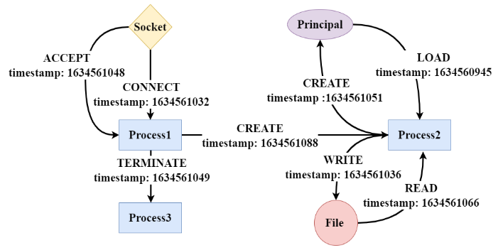
This article considers log events about files (e.g. file creation, file reading, file writing), processes (e.g. creation and permission changes), network sockets (e.g. network connections), principals (users or accounts), etc. An edge consists of events that describe actions performed by a source entity on a target entity (for example, a process reads a file). Figure 2 shows an example.

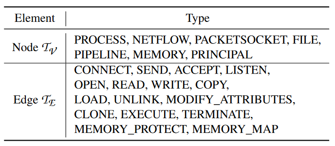
The complete list of node types and edge types considered by PROGRAPHER is shown in Table 2.

To efficiently handle large amounts of incoming logs, PROGRAPHER builds time-ordered snapshots. As logs are ingested, it maintains a cached graph. For each incoming log, when the event source and target are not visible, they are added as nodes to the cache graph, an edge is also created between the pair of new nodes, and the log timestamp is assigned to these nodes. For an existing pair of nodes, their timestamps are updated. When the number of nodes reaches n (also called snapshot size), all n nodes and their edges are saved into the first snapshot. Afterwards, PROGRAPHER adds new nodes from the incoming log, uses the forgetting rate (fr) to evict the $n × fr$ oldest nodes, and saves the cached graph to a new snapshot when the number of nodes reaches $n × (1 + fr)$. This makes a pair of adjacent snapshots always have $n × (1 − fr) $overlapping in the node.

Repeat this process to generate a series of snapshots ${S_1, S_2,…, S_k}$. With such a design, it is ensured that temporal dynamics can be recovered by comparing adjacent snapshots, and that the size of each snapshot is controlled. Furthermore, the ratio between benign and malicious traces in a snapshot is expected to be much smaller than the entire provenance graph, thus addressing the data imbalance problem. The pseudocode is shown in Algorithm 1.

# Encoder

(1) Enumerate each node to extract RSGs of different degrees, thereby capturing the node’s neighborhood information. In graph2vec, this is achieved by utilizing Weisfeiler-Lehman (WL) graph kernels to test graph isomorphism. Specifically, for a node v, the WL kernel takes its label and the labels of its connected edges and nodes as input labels, and then, generates a new label for v aggregated from the input labels, called RSG. The entire process is repeated d times on each node $ v ∈ V $ to describe its neighborhood of depth $1, …, d $ .

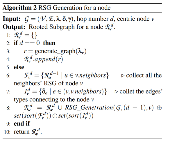
To adapt to the format of the provenance graph, this paper treats node and edge types as labels (the original WL kernel only considers node types). In addition, the authors found that RSGs generated from large and dense graphs may have many redundant labels. To improve efficiency, this paper only retains the unique labels of each RSG. The steps of RSG generation are described in Algorithm 2. As a specific example, the RSG of node “Process2” when d = 0, 1, 2 in Figure 2 is:

• d = 0: [(Process)].
• d = 1: [(Process), (File), (Principal), LOAD, WRITE, CREATE, READ].
• d = 2: [(Process, File, Principal, LOAD, WRITE, CREATE, READ), (Process, Principal, LOAD, CREATE), (Process, File, READ, WRITE), (Process, Socket, CREATE, CONNECT, TERMINATE, ACCEPT), LOAD, WRITE, CREATE, READ].

(2) Generate embedding $E_{S_i}$ of snapshot $S_i$. $E_{S_i}$ is initialized as a random vector and then updated by maximizing the log-likelihood of the RSG of all nodes, which are also represented by embeddings. The embeddings E of all snapshots ${S_1, S_2,…, S_k}$ can be updated together via gradient descent. The update process follows the skipgram model used by doc2vec. Define the objective function as:

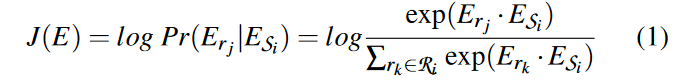
For training efficiency, this paper applies negative sampling like previous work based on unsupervised learning. On snapshot $S_i$, m RSGs $R ′ _i= {r_1, r_2, ··· , r_m}$ are randomly selected from the entire sub-graph set as negative samples, such that $R′_i\cap R_i \neq 0$. The objective function J(E ) will be adjusted to maximize the log-likelihood of $R_i $ and simultaneously minimize the log-likelihood of $R′_i$ . Since $R′_i$ is a subset of non-existent RSG, the training overhead is reduced. The entire process of embedding generation is summarized in Algorithm 3.

# Anomaly Detector

After generating a representation of the snapshot, PROGRAPHER proceeds to detect anomalous snapshots. Considering changes between snapshots as important inputs for detection, and examining the snapshot sequence ${S_1, S_2,…, S_k}$ together, the bidirectional recurrent structure and convolutional neural network model proposed by TextRCNN, which has been widely used for text classification, was selected for this task.

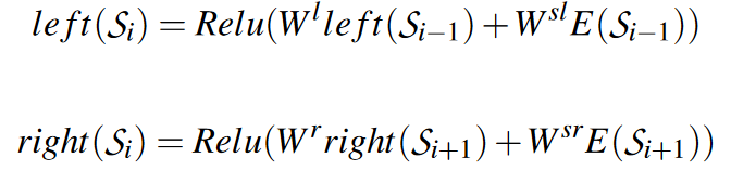
To train an anomaly detector, we take as input a set of snapshot sequences and their associated embeddings. Use recurrent structures and convolutional networks to obtain the latent representation $y_i$ of each snapshot $S_i$ in the input sequence, which is defined as follows:

where $x_i=[left(S_i);E(S_i);right(S_i)]$ is the concatenation of the left context vector, its own embedding and the right context vector. W is the weight matrix and b is the bias vector. The left and right context vectors are defined as:

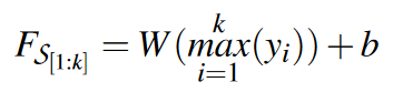
Utilize maxpool layer and fully connected layer to obtain the final representation of each snapshot sequence

During the training phase, given a snapshot sequence ${S_1,S_2,…, S_k}$, we predict how likely it is that the sequence is related to its subsequent snapshot $S_{k+1}$. Define the loss as the distance of L2 distance as follows:

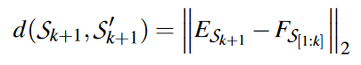
where $E_{S_{k+1}}$ is the embedding of snapshot $S_{k+1}$. In the testing phase, given a sequence of snapshots, its predicted embedding is compared with the true embedding. If the distance between them exceeds a predefined threshold, they are marked as anomalies.

# Key Indicator Generator

When an anomalous snapshot is detected, key indicators of malicious activity are generated. The author found that other works such as Unicorn were missing this step. Therefore, their detection results are coarse-grained. But with the adoption of graph2vec, PROGRAPHER can achieve more fine-grained attack attribution.

The objective function J(E) measures the co-occurrence probability between the snapshot embedding and each RSG, and the smaller its value, the smaller the co-occurrence probability. Since the likelihood is calculated against each RSG of the snapshot, it is possible to sort the RSGs by their probability and select key indicators from them. In particular, during the testing phase, given a snapshot $S_i$, the embedding $E_{S_i}$ generated from $S_i$ is compared with the embedding $E’_{S_i}$ predicted from a sequence of k snapshots, and the difference between the two embeddings for each RSG is extracted. After that, the RSGs are sorted according to the loss difference and the top K suspicious RSGs are selected. RSG can be mapped to multiple nodes because it only stores node and edge types. Therefore, the system searches the snapshot to find all nodes matching the K suspicious RSGs and feeds them back to the analyst.

# Experiment development and results

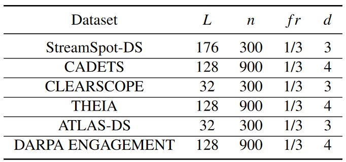
To ensure that each snapshot contains enough information to learn its representation, the authors set the snapshot size n according to the size of the dataset. For small graphs with less than 10K nodes (such as a traceability graph for software on a machine), n is set to 300. For large graphs with more than 10k nodes (such as operating system provenance graphs), n is set to 900. For different datasets, L is configured as 32, 128, and 176. During snapshot construction, use the forgetting rate fr set to 1/3. For the encoder and anomaly detector, this paper selects hyperparameters through grid search, and their optimal values ​​are described in Table 3 below.

Training and testing are performed on a server equipped with a 32-core Intel E5-2640 processor, 256 GB physical memory and 1 Nvidia GTX TITAN X GPU, and the operating system is Ubuntu 14.04.6 LTS.

# Dataset

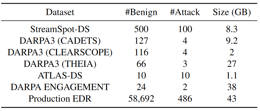
This paper uses two log datasets with simulated attacks (StreamSpot and ATLAS) and two DARPA datasets (DARPA3 and DARPA ENGAGEMENT) to evaluate the real-world performance of PROGRAPHER. In addition, this article deploys PROGRAPHER in a production environment to analyze system logs collected by commercial EDR products. As shown in the data set statistics shown in Table 4 below, “#Benign” and “#Attack” are the number of benign graphs and attack graphs. Sizes are measured on preprocessed plots, not raw data. Each dataset is separated by training, validation and testing, and in the experiments it is ensured that all datasets are disjoint and that all benign plots in the test set occur after the training and validation plots.

# Effectiveness evaluation

Table 5 shows the experimental results of Sreamspot-DS and DARPA3 under 100 repeated experiments. Taking Unicorn as the baseline, the ProGrapher method in this article has better performance in precision, recall, accuracy and F1 value.

Unicorn results are worse than those reported in the paper, mainly due to:

1. I learned from the Unicorn author that they used a non-public benign data set under DARPA TC for training, and the author of this article does not have access to this data set.
2. The Unicorn implementation does not force graphs under test to occur after training and validation, which is a common “data snooping” problem in security systems [5].

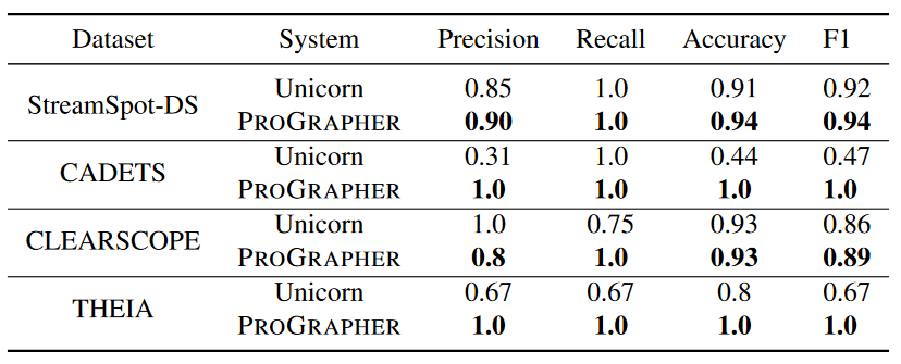
Only one benign graph in CLEARSCOPE was incorrectly detected as an anomaly. FP is mainly caused by insufficient behavioral information in the training set. Since the authors only keep the latest events for the same pair of entities, for CLEARSCOPE, hundreds of events can be deleted for each entity pair. This strategy removes useful information that can distinguish benign from malicious behavior, which explains why the size of the CLEARSCOPE dataset after preprocessing is small (only 2GB).

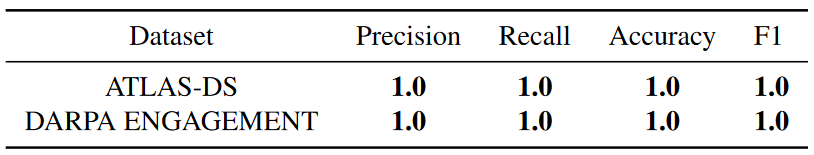
Table 6 shows the performance of ProGrapher on the ATLAS-DS and DARPA ENGAGEMENT data sets. The ProGrapher system successfully detected all attacks and did not generate any FP. The results also show that PROGRAPHER can handle different types of APT attacks.

Experimental results in Production EDR. Approximately 59K charts were extracted from 180GB of logs by endpoint. Starting from the first 7 days, the authors use 51119 benign graphs for training (benign graphs are selected by analysts) and 2889 benign graphs for validation. In the remaining 2 days, we used 4684 benign graphs and 486 attack graphs for testing.

In Figure 3, the authors draw a ROC curve to illustrate the relationship between TPR and FPR and compare it with Unicorn. The results show that PROGRAPHER can achieve reasonable accuracy in a production environment, such as 94% TPR, 14% FPR. The detection accuracy of Unicorn is significantly lower than PROGRAPHER, e.g., at 20% FPR, the TPR is lower than 10%. The area under the curve (AUC) of PROGRAPHER is almost twice that of Unicorn (0.943 vs. 0.542).

# Generate indicator evaluation

**Indicator validity. ** The ProGrapher method selects the top K RSGs from the exception snapshot and feeds back all nodes matching these RSGs. Given a real attacking node, we consider nodes in the 3-hop neighborhood to be valid and all other nodes to be invalid.

The 3-hop neighborhood is chosen in this article because the WL kernel depth of the small graph is set to 3 in this article (4 for the large graph), because it is a common practice to investigate neighborhood entities when an alert is given, and the metric is considered valid if at least one node in the metric belongs to the attacking node or a valid neighbor.

Effectiveness is calculated as the ratio between effective metrics and all metrics identified by PROGRAPHER. Table 7 shows the ratios for different K (from 1 to 5) for the 3 DARPA3 subsets. It can be seen that even if the K value is between 2 and 3, the efficiency is already quite high (at least 0.94).

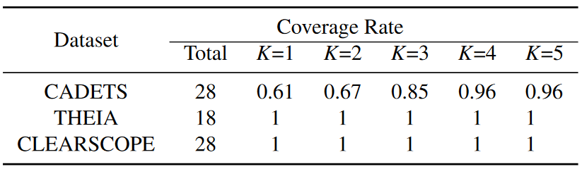
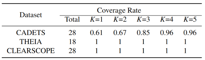
Define coverage as the ratio between correctly identified attack nodes and all real attack nodes. Table 8 shows the coverage for each dataset for K ranging from 1 to 5. For THEIA and CLEARSCOPE datasets, all attack nodes are identified, and for CADETS, only 1 attack node is lost when K ≥ 4.

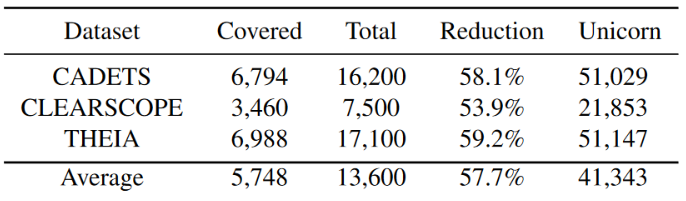
Define the reduction ratio as 1 − Covered/Total (“Covered” and “Total” are the number of nodes mapped to all indicators and the number of all nodes in the exception snapshot). Table 9 shows the workload reduction for each DARPA3 dataset when K = 4. On average, Metrics Generator reduces security analysts’ workload by 58%. In contrast, the baseline system Unicorn only tells if a snapshot is abnormal, and analysts must investigate all included nodes. We summed the number of nodes for all alert snapshots of Unicorn and display it in Table 10. The number of nodes to be investigated in Unicorn is 41343, which is 7.1 times that of PROGRAPHER.

Unicorn’s value is higher than Total because Unicorn predicts larger snapshots as anomalies

# Run performance evaluation

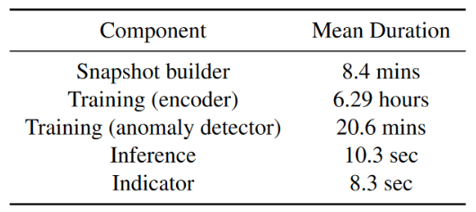
The runtime overhead of each component is shown in Table 10, and the results are the average of repeated runs on different DARPA3 datasets.

**Data processing and training. ** On average, PROGRAPHER takes 8.4 minutes to process one day’s worth of logs from a dataset and 8.3 microseconds to generate the snapshot sequence. PROGRAPHER takes 6.29 hours to train the encoder model for 100 epochs. For the anomaly detector, training takes approximately 20.6 minutes.

**Inference and indicator generation. ** PROGRAPHER takes an average of 10.3 seconds to predict anomaly snapshots and 8.3 seconds to generate a sorted RSG for each anomalous snapshot.

Demonstrates that PROGRAPHER is capable of near real-time anomaly detection

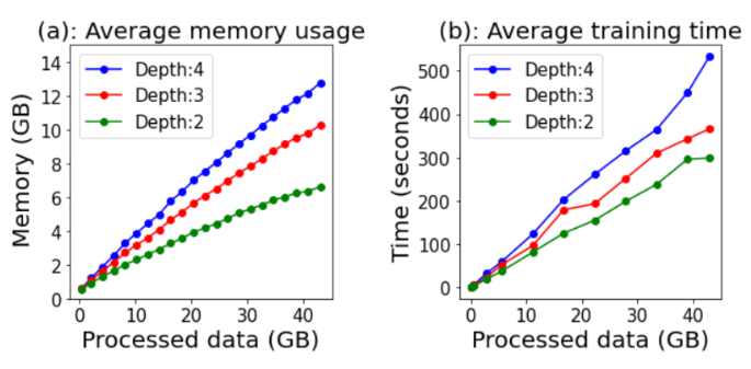
**Scalability. ** This article first measures how memory consumption increases with the amount of data by changing the number of training graphs. For the same data size, the depth (d) of the WL kernel has the greatest impact, so changing its value from 2 to 4, Figure 4(a) shows the relationship between data volume and memory consumption. Because PROGRAPHER performs training and inference on snapshots rather than the entire dataset, memory consumption scales sublinearly with the amount of data. For example, even when processing 40 GB of data with d set to 4, the maximum memory usage is 12.7 GB, of which 10.2 GB is used for training and storing embeddings. The time consumption of each epoch is shown in Figure 6(b). The time consumption has a linear relationship with the amount of data. Only when d = 4 and the data size exceeds 30GB, the time consumption increases faster.

# Other experiments

This paper uses the relatively small dataset StreamSpot-DS (8.3GB) to analyze the impact of key parameters on the effectiveness of PROGRAPHER. Using the ATLAS-DS dataset, PROGRAPHER is tested for robustness by emulating an evasion attack by inserting many random events before and after the attack event.

# Research trends

**Change in normal behavior. ** Because PROGRAPHER is designed as an anomaly detection system on provenance graphs, it will alert when unseen behavior is observed. However, changes in normal behavior (for example, an employee logging into a new internal server) may be viewed as an anomaly, which may introduce false positives. This problem can be viewed as a concept drift problem, which can be partially mitigated by retraining PROGRAPHER using updated data. It is crucial to detect when concept drift occurs so that frequent and costly retraining does not need to be performed.

**Inductive and inductive learning. ** The current design of PROGRAPHER follows a push-through learning model, assuming that all RSGs in the test phase have been seen in the training phase. PROGRAPHER must be retrained when a new RSG is encountered. Although this article reduces the chance of seeing new RSGs by building them using only node and edge types, retraining will still be required in a production environment. This limitation also exists in existing graph learning-based security systems such as Euler and ShadeWatcher. To address this issue, future research could explore inductive learning models that are capable of dynamically generating embeddings for new nodes from their neighborhoods without retraining. However, in this case, a different encoder model must be chosen, such as GraphSage.

**More adaptive attacks. ** An effective countermeasure is to inject repeated events to fill the cache used to build snapshots. In the experiments of this article, it was found that the false negatives on the CLEARSCOPE dataset are caused by event aggregation. This problem exists in other event aggregation traceability systems (such as ShadeWatcher). One possible solution is to retain more information after event aggregation (e.g. distribution of certain event fields).

# Comparative analysis of literature

# Learning-based traceability analysis

When the target is an edge/node, the trained system aims to determine whether the interaction between a pair of entities or the entities themselves are malicious. ShadeWatcher builds a knowledge graph based on system logs and uses a graph neural network (GNN)-based recommendation system to detect malicious interactions. SIGL leverages node embeddings and autoencoder models to determine whether a process generated from a Software Installation Graph (SIG) is malicious. However, when encountering large traceability graphs, it is quite challenging to achieve high-precision edge/node-based detection. Furthermore, detection results do not provide contextual information that is valuable for understanding attack activity (e.g., other activities related to the detected edge/node).

However, the Flash article stated that ShadeWatcher can provide context-related information.

ShadeWatcher achieves high detection accuracy, but it is evaluated on small graphs (most graphs have only a few hundred interactions)

The SIG checked by SIGL is usually very small

For path-based detection, paths that match certain patterns (e.g., associated with POI nodes) are selected from the source graph, and the trained system classifies the paths. For example, ProvDetector identifies covert malware by applying word embeddings to convert execution paths into vectors and then clustering them. Atlas applies lemmatization and word embeddings to generate sequences, and uses a long short-term memory (LSTM) network to predict whether a sequence is relevant to an attack. However, these methods first rely on heuristics to select POI paths (ProvDetector selects rare paths customized for stealth malware) or nodes (ATLAS assumes some malicious nodes are known) and then apply learning-based methods.

For graph-based detection, the provenance graph is either classified as a whole or decomposed into a set of subgraphs, and classification is performed on these subgraphs. For example, Unicorn slices logs through sliding time windows and constructs evolutionary subgraphs from them. For each subgraph, graph sketching converts the histogram capturing structural features into a fixed-size vector. ProvGem proposes multiple embeddings to capture different contexts of nodes and classify graphs on aggregated node embeddings in a supervised learning manner. The main problem with graph-based detection is that its detection granularity is too coarse, and analysts still need to expend considerable effort to pinpoint malicious entities/events from graphs that may include thousands of nodes.

HERCULE uses a semi-supervised community detection algorithm to correlate attack events and reconstruct attacks. Streamspot extracts local graph features through breadth-first search (BFS) and clusters snapshots to detect abnormal features. P-Gaussian applies the Gaussian distribution principle to calculate the similarity between intrusion behaviors and their variants. Log2vec builds heterogeneous graphs from logs and applies graph embeddings to detect anomalous activities.

# Heuristic-based traceability analysis

Heuristic-based origin analysis. To address the “dependency explosion” problem, another direction is to apply manually written rules to prioritize investigations. Many previous works perform graph traversal (e.g., breadth-first search) from POI events and select suspicious paths based on the rules. For example, NoDoze uses historical information to assign threat scores to alerts in a provenance graph and then identifies anomalous paths. PrioTracker accelerates forward tracking by calculating the event’s rarity score to prioritize unusual events. Padoga considers the degree of anomaly of individual paths and the entire provenance graph to identify intrusions. SLEUTH and Morse use label-based information flow techniques to reconstruct attack scenarios.

Analysts query the provenance graph using attack signatures, such as indicators of compromise (IoCs), and analyze similar subgraphs. $\tau$-calculus proposes a new domain-specific language (DSL) to make querying for threat analysts more intuitive and efficient. The Poirot model models this problem as a graph pattern matching (GPM) problem and proposes a new graph alignment method for it.

Some works extract summary graphs from fine-grained source graphs to simplify investigation. RapSheet and Holmes rely on a knowledge base of adversarial tactics, techniques, and procedures (TTPs) to build summary graphs. DepComm summarizes process-centric community-based provenance graphs and extracts information paths for attack investigation.

# Log anomaly detection

PROGRAPHER relies on graph2vec, which uses NLP technologies such as doc2vec and word2vec for graph embedding. Similar NLP technology is also used to detect abnormal logs. Deeplog treats audit logs as sentences and leverages LSTM models to detect abnormal events. LogAnomaly applies word2vec to extract semantic information hidden in log templates to detect log anomalies. Attack2Vec uses temporal word embeddings to model and track the evolution of attack steps.

# reference

This section only lists the references that I think are important and closely related to the work of this article.

[1] Abdulellah Alsaheel, Yuhong Nan, Shiqing Ma, Le Yu, Gregory Walkup, Z. Berkay Celik, Xiangyu Zhang, and Dongyan Xu. ATLAS: A sequence-based learning approach for attack investigation. In Michael Bailey and Rachel Greenstadt, editors, USENIX Security Symposium, pages 3005–3022. USENIX Association, 2021.

[2] Xueyuan Han, Thomas F. J.-M. Pasquier, Adam Bates, James Mickens, and Margo I. Seltzer. UNICORN: runtime provenance-based detector for advanced persistent threats. CoRR, abs/2001.01525, 2020.

[3] Qi Wang, Wajih Ul Hassan, Ding Li, Kangkook Jee, Xiao Yu, Kexuan Zou, Junghwan Rhee, Zhengzhang Chen, Wei Cheng, Carl A. Gunter, and Haifeng Chen. You are what you do: Hunting stealthy malware via data provenance analysis. In NDSS. The Internet Society, 2020.

[4] J. Zeng, X. Wang, J. Liu, Y. Chen, Z. Liang, T. Chua, and Z. Chua. Shadewatcher: Recommendation-guided cyber threat analysis using system audit records. In 2022 IEEE Symposium on Security and Privacy (SP) (SP), 2022.

[5] Daniel Arp, Erwin Quiring, Feargus Pendlebury, Alexander Warnecke, Fabio Pierazzi, Christian Wressnegger, Lorenzo Cavallaro, and Konrad Rieck. Dos and don’ts of machine learning in computer security. In Proc. of the USENIX Security Symposium, 2022.

[6] Wajih Ul Hassan, Adam Bates, and Daniel Marino. Tactical provenance analysis for endpoint detection and response systems. In IEEE Symposium on Security and Privacy, pages 1172–1189. IEEE, 2020.

[7] Sadegh Momeni Milajerdi, Rigel Gjomemo, Birhanu Eshete, R. Sekar, and V. N. Venkatakrishnan. HOLMES: real-time APT detection through correlation of suspicious information flows. In IEEE Symposium on Security and Privacy, pages 1137–1152. IEEE, 2019.

[8] Z. Xu, P. Fang, C. Liu, X. Xiao, Y. Wen, and D. Meng. Depcomm: Graph summarization on system audit logs for attack investigation. In 2022 2022 IEEE Symposium on Security and Privacy (SP) (SP), 2022.

# Original statement

This article is my UCAS course paper reading report and is not allowed to be reproduced! ! !

This article is my UCAS course paper reading report and is not allowed to be reproduced! ! !

This article is my UCAS course paper reading report and is not allowed to be reproduced! ! !